hamiltorch: a PyTorch Python package for sampling

What is hamiltorch?

hamiltorch is a Python package that uses Hamiltonian Monte Carlo (HMC) to sample from probability distributions. As HMC requires gradients within its formulation, we built hamiltorch with a PyTorch backend to take advantage of the available automatic differentiation. Since hamiltorch is based on PyTorch, we ensured that hamiltorch is able to sample directly from neural network (NN) models (objects inheriting from the torch.nn.Module). As far as we are aware there are two main strengths to hamiltorch:

We have built Riemannian Manifold Hamiltonian Monte Carlo into our framework, which allows others to build/improve on the possible Riemannian metrics available in our toolbox.
Anyone can build a NN model in PyTorch and then use hamiltorch to directly sample from the network. This includes using Convolutional NNs and taking advantage of GPUs.

Getting started

Go to hamiltorch

git clone https://github.com/AdamCobb/hamiltorch.git
cd hamiltorch
pip install .

Now you are ready to start playing around with hamiltorch.

We can start with opening up a Jupyter Notebook and importing the relevant modules:

import torch
import hamiltorch
import matplotlib.pyplot as plt
%matplotlib inline

We can also take this opportunity to use hamiltorch to set the random seed and select a GPU if it is available (however I recommend sticking to CPU(s) unless you are working on a large NN e.g. see here).

hamiltorch.set_random_seed(123)
device = torch.device('cuda' if torch.cuda.is_available() else 'cpu')

Now we are ready to introduce an application:

Sampling a multivariate Gaussian

We would like to sample from a multivariate Gaussian distribution. However, we cannot directly sample from the distribution as one normally would. The task is to use hamiltorch to sample from this multivariate Gaussian.

This is where I introduce one of the core components of hamiltorch, the log probability function. In hamiltorch, we have designed the samplers to receive a function handle log_prob_func, which the sampler will use to evaluate the log probability of each sample. A log_prob_func must take a 1-d vector of length equal to the number of parameters that are being sampled. For the example of our multivariate Gaussian distribution, we can define our log_prob_func as follows:

def log_prob_func(params):
    mean = torch.tensor([1.,2.,3.])
    stddev = torch.tensor([0.5,0.5,0.5])
    return torch.distributions.Normal(mean, stddev).log_prob(params).sum()

This simply defines the log probability of a 3-dimensional Gaussian distribution, \(\mathcal{N}(\mathbf{x};\boldsymbol{\mu},\boldsymbol{\Sigma})\), where \(\boldsymbol{\mu} = [1,2,3]\) and \(\boldsymbol{\Sigma} = \mathrm{diag}([0.5,0.5,0.5])\). Therefore for a 3-dimensional vector, log_prob_func returns a single number corresponding to \(p(\mathbf{x}\vert\boldsymbol{\mu},\boldsymbol{\Sigma})\).

Now that the log_prob_func has been defined above, we can start to use the core sampler in hamiltorch. Here, I introduce the hamiltorch.sample function, where details of the arguments and their definitions are listed here. We can now sample from the multivariate Gaussian using mostly the default sampler settings (Standard HMC). This is without spending too much time optimising the parameters such as the trajectory length (num_steps_per_sample) and the step size.

Simple HMC:

num_samples = 400
step_size = .3
num_steps_per_sample = 5

hamiltorch.set_random_seed(123)
params_init = torch.zeros(3)
params_hmc = hamiltorch.sample(log_prob_func=log_prob_func, params_init=params_init,  num_samples=num_samples, step_size=step_size, num_steps_per_sample=num_steps_per_sample)

Output:

Sampling (Sampler.HMC; Integrator.IMPLICIT)
Time spent  | Time remain.| Progress             | Samples | Samples/sec
0d:00:00:00 | 0d:00:00:00 | #################### | 400/400 | 506.48       
Acceptance Rate 1.00

Riemannian HMC:

Say we now want to perform Riemannian Manifold HMC (RMHMC), which incorporates the geometry of the problem. We can simply select RMHMC by setting sampler=hamiltorch.Sampler.RMHMC.

sampler=hamiltorch.Sampler.RMHMC
integrator=hamiltorch.Integrator.IMPLICIT

hamiltorch.set_random_seed(123)
params_init = torch.zeros(3)
params_irmhmc = hamiltorch.sample(log_prob_func=log_prob_func, params_init=params_init, num_samples=num_samples, step_size=step_size, num_steps_per_sample=num_steps_per_sample, sampler=sampler, integrator=integrator)

Output:

Sampling (Sampler.RMHMC; Integrator.IMPLICIT)
Time spent  | Time remain.| Progress             | Samples | Samples/sec
0d:00:00:29 | 0d:00:00:00 | #################### | 400/400 | 13.73       
Acceptance Rate 1.00

We can also repeat the above RMHMC scheme for explicit integration and set the integrator=hamiltorch.Integrator.EXPLICIT. For the differences between the integrators and the samplers, please refer to our paper.

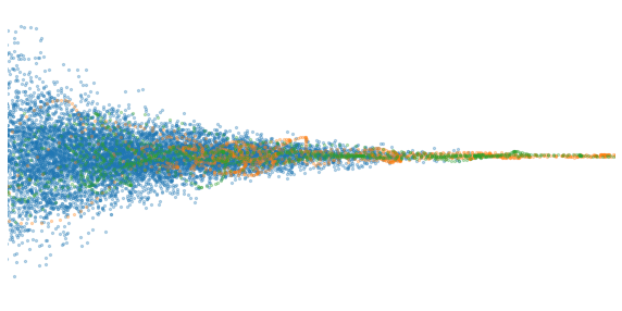
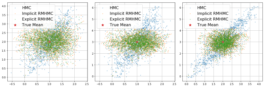
We can then plot these 3D samples below.

_{Samples taken from the 3D Gaussian distribution plotted in three 2D plots.} _{Both Riemannian-based samplers benefit from taking into account the underlying geometry.}

Sampling from a more complicated distribution

So far we have sampled from a simple multivariate Gaussian distribution, where the geometry was well defined such that the metric tensor is always positive semi-definitive. In order to give a flavour of how one might go about dealing with less-well behaved log probabilities, we will use the funnel distribution¹ as an illustrative example.

Definition:

\[\prod_i^D\mathcal{N}(x_i\vert 0, \exp\{-v\})\mathcal{N}(v\vert 0, 3^2)\]

Where we wish to sample the \(D+1\) dimensional vector \([v, x_1, \dots x_D]\).

Code for log_prob_func:

D = 10
# log_prob_func for funnel
def funnel_ll(w, dim=D):
    v_dist = torch.distributions.Normal(0,3)
    ll = v_dist.log_prob(w[0])
    x_dist = torch.distributions.Normal(0,torch.exp(-w[0])**0.5)
    ll += x_dist.log_prob(w[1:]).sum()
    return ll

The key reason for using the funnel distribution is because its marginal distribution, \(p(v) = \mathcal{N}(v\vert 0, 3^2)\), is a simple Gaussian. Therefore, despite it being a hierarchical model that is challenging to sample, the marginal is known and can be compared with the empirical samples.

The problem we have now is that the metric tensor is no longer positive semi-definitive. A possible solution to this problem is by filtering out the negative eigenvalues using softabs². This can be done by setting metic=hamiltorch.Metric.SOFTABS for all RMHMC samplers.

Again, we can now run the three different samplers as follows:

Simple HMC:

hamiltorch.set_random_seed(123)
params_init = torch.ones(D + 1)
params_init[0] = 0.
step_size = 0.3093
num_samples = 500
L = 25
omega=100
threshold = 1e-3
softabs_const=10**6

params_hmc = hamiltorch.sample(log_prob_func=funnel_ll, params_init=params_init, num_samples=num_samples,
                               step_size=step_size, num_steps_per_sample=L)

Output:

Sampling (Sampler.HMC; Integrator.IMPLICIT)
Time spent  | Time remain.| Progress             | Samples | Samples/sec
0d:00:00:10 | 0d:00:00:00 | #################### | 500/500 | 45.89       
Acceptance Rate 0.99

Implicit RMHMC:

hamiltorch.set_random_seed(123)
params_init = torch.ones(D + 1)
params_init[0] = 0.
step_size = 0.15
num_samples = 50
num_steps_per_sample = 25
threshold = 1e-3
softabs_const=10**6

params_i_rmhmc = hamiltorch.sample(log_prob_func=funnel_ll, params_init=params_init, num_samples=num_samples,
                                   sampler=hamiltorch.Sampler.RMHMC, integrator=hamiltorch.Integrator.IMPLICIT,
                                   metric=hamiltorch.Metric.SOFTABS, fixed_point_threshold=threshold, jitter=0.01,
                                   num_steps_per_sample=num_steps_per_sample, step_size=step_size, softabs_const=softabs_const)

Output:

Note that as the funnel distribution can be ill-defined in some parts of the space, the sampler informs the user when a sample results in an invalid log probability or an invalid hessian. These samples are rejected and the sampler recovers and continues from the previous accepted sample.

    Sampling (Sampler.RMHMC; Integrator.IMPLICIT)
    Time spent  | Time remain.| Progress             | Samples | Samples/sec
    Invalid log_prob: -inf, params: tensor([ -190.1948, -2425.3206,  -269.3571, -2584.8828,  -853.4375, -1716.3528,
            -1671.2803,  1183.8041, -1716.4843,   -13.2883,   396.5518],
           grad_fn=<AddBackward0>)
    Invalid hessian: tensor([[       nan, -0.0000e+00, -0.0000e+00, -0.0000e+00, -0.0000e+00, -0.0000e+00,
             -0.0000e+00, -0.0000e+00, -0.0000e+00, -0.0000e+00, -0.0000e+00],
            [-0.0000e+00, 1.1894e-33, -0.0000e+00, -0.0000e+00, -0.0000e+00, -0.0000e+00,
             -0.0000e+00, -0.0000e+00, -0.0000e+00, -0.0000e+00, -0.0000e+00],
            [-0.0000e+00, -0.0000e+00, 1.1894e-33, -0.0000e+00, -0.0000e+00, -0.0000e+00,
             -0.0000e+00, -0.0000e+00, -0.0000e+00, -0.0000e+00, -0.0000e+00],
            [-0.0000e+00, -0.0000e+00, -0.0000e+00, 1.1894e-33, -0.0000e+00, -0.0000e+00,
             -0.0000e+00, -0.0000e+00, -0.0000e+00, -0.0000e+00, -0.0000e+00],
            [-0.0000e+00, -0.0000e+00, -0.0000e+00, -0.0000e+00, 1.1894e-33, -0.0000e+00,
             -0.0000e+00, -0.0000e+00, -0.0000e+00, -0.0000e+00, -0.0000e+00],
            [-0.0000e+00, -0.0000e+00, -0.0000e+00, -0.0000e+00, -0.0000e+00, 1.1894e-33,
             -0.0000e+00, -0.0000e+00, -0.0000e+00, -0.0000e+00, -0.0000e+00],
            [-0.0000e+00, -0.0000e+00, -0.0000e+00, -0.0000e+00, -0.0000e+00, -0.0000e+00,
             1.1894e-33, -0.0000e+00, -0.0000e+00, -0.0000e+00, -0.0000e+00],
            [-0.0000e+00, -0.0000e+00, -0.0000e+00, -0.0000e+00, -0.0000e+00, -0.0000e+00,
             -0.0000e+00, 1.1894e-33, -0.0000e+00, -0.0000e+00, -0.0000e+00],
            [-0.0000e+00, -0.0000e+00, -0.0000e+00, -0.0000e+00, -0.0000e+00, -0.0000e+00,
             -0.0000e+00, -0.0000e+00, 1.1894e-33, -0.0000e+00, -0.0000e+00],
            [-0.0000e+00, -0.0000e+00, -0.0000e+00, -0.0000e+00, -0.0000e+00, -0.0000e+00,
             -0.0000e+00, -0.0000e+00, -0.0000e+00, 1.1894e-33, -0.0000e+00],
            [-0.0000e+00, -0.0000e+00, -0.0000e+00, -0.0000e+00, -0.0000e+00, -0.0000e+00,
             -0.0000e+00, -0.0000e+00, -0.0000e+00, -0.0000e+00, 1.1894e-33]],
           grad_fn=<DivBackward0>), params: tensor([ -75.8118, -503.8369, -120.8768, -207.3312,  252.1230, -685.7836,
            -530.2316, -203.5684,  192.2168,  -27.8746, -715.1514],
           grad_fn=<AddBackward0>)
    Invalid log_prob: -inf, params: tensor([ -104.7945, -1396.6093, -1758.9779,   490.2879,  -305.7715,  -188.9097,
             -176.8809,   378.2602,    99.7805,   913.4412,   272.1174],
           grad_fn=<AddBackward0>)
    0d:00:14:53 | 0d:00:00:00 | #################### | 50/50 | 0.06       
    Acceptance Rate 0.94

Explicit RMHMC:

hamiltorch.set_random_seed(123)
params_init = torch.ones(D + 1)
params_init[0] = 0.
step_size = 0.15
num_samples = 50
num_steps_per_sample = 25
explicit_binding_const=10
softabs_const=10**6

params_e_rmhmc = hamiltorch.sample(log_prob_func=funnel_ll, params_init=params_init, num_samples=num_samples,
                                   sampler=hamiltorch.Sampler.RMHMC, integrator=hamiltorch.Integrator.EXPLICIT,
                                   metric=hamiltorch.Metric.SOFTABS, fixed_point_threshold=threshold, jitter=0.01,
                                   num_steps_per_sample=num_steps_per_sample, step_size=step_size, explicit_binding_const=explicit_binding_const,
                                   softabs_const=softabs_const)

Output:

Sampling (Sampler.RMHMC; Integrator.EXPLICIT)
Time spent  | Time remain.| Progress             | Samples | Samples/sec
Invalid hessian: tensor([[nan, -inf, inf, -inf, -inf, -inf, -inf, -inf, -inf, -inf, -inf],
        [-inf, nan, nan, nan, nan, nan, nan, nan, nan, nan, nan],
        [inf, nan, nan, nan, nan, nan, nan, nan, nan, nan, nan],
        [-inf, nan, nan, nan, nan, nan, nan, nan, nan, nan, nan],
        [-inf, nan, nan, nan, nan, nan, nan, nan, nan, nan, nan],
        [-inf, nan, nan, nan, nan, nan, nan, nan, nan, nan, nan],
        [-inf, nan, nan, nan, nan, nan, nan, nan, nan, nan, nan],
        [-inf, nan, nan, nan, nan, nan, nan, nan, nan, nan, nan],
        [-inf, nan, nan, nan, nan, nan, nan, nan, nan, nan, nan],
        [-inf, nan, nan, nan, nan, nan, nan, nan, nan, nan, nan],
        [-inf, nan, nan, nan, nan, nan, nan, nan, nan, nan, nan]],
       grad_fn=<DivBackward0>), params: tensor([  75.5394,  -10.3087,    8.2127,  -20.3933,  -65.2353,  -19.7363,
         -21.4557,  -35.2749, -160.6523,  -34.1107,   -5.9985],
       requires_grad=True)
Invalid log_prob: -inf, params: tensor([-168.7018,   36.5917,  -56.3353,  -68.8884,   92.6008,   63.7991,
          40.8584,   50.6511,   10.5664,  -41.6701,  -45.2683],
       requires_grad=True)
0d:00:03:27 | 0d:00:00:00 | #################### | 50/50 | 0.25       
Acceptance Rate 0.94

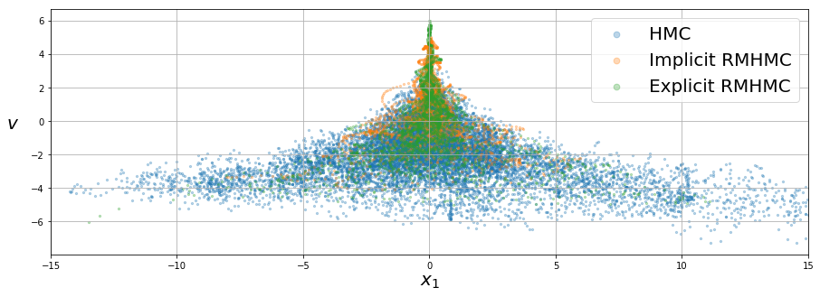
We can then plot the samples (selecting one of the \(D\) \(x_i\)’s to be on the horizontal axis):

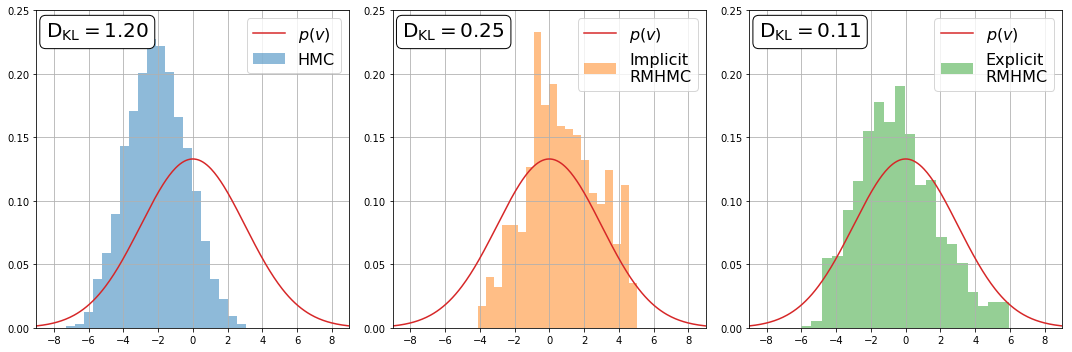
_{Samples taken from the 11-dimensional funnel distribution.} _{Again, both Riemannian-based samplers benefit from taking into account the underlying geometry and are able to sample in the narrow part of the funnel.}

We can also plot the marginal distributions of \(v\) by representing them in histograms. We plot the known Gaussian distribution in each figure for comparison. The KL divergence, \(\mathrm{D_{KL}}\), is also included to measure how close the empirical distribution is from the true one.

_{The marginal distributions of all three samplers.} _{Compared to the known distribution (the red line), the Riemannian samplers provide samples that appear less biased by the narrowness of the funnel. This leads to a lower (better) KL divergence.}

Bayesian neural networks with hamiltorch

We have built hamiltorch in a way that makes it easy to run HMC over any network. Rather than needing to define the appropriate likelihood and priors for the network, we have already built a specific function, hamiltorch.sample_model, that wraps around hamiltorch.sample and does all this for you. For example, let’s define a PyTorch convolutional neural network (CNN)³, which has been designed for the MNIST data set⁴ as follows:

import torch.nn as nn
import torch.nn.functional as F
hamiltorch.set_random_seed(123)
device = torch.device('cuda' if torch.cuda.is_available() else 'cpu')
class Net(nn.Module):
    """ConvNet -> Max_Pool -> RELU -> ConvNet -> Max_Pool -> RELU -> FC -> RELU -> FC -> SOFTMAX"""
    def __init__(self):
        super(Net, self).__init__()
        self.conv1 = nn.Conv2d(1, 20, 5, 1)
        self.conv2 = nn.Conv2d(20, 50, 5, 1)
        self.fc1 = nn.Linear(4*4*50, 500)
        self.fc2 = nn.Linear(500, 10)

    def forward(self, x):
        x = F.relu(self.conv1(x))
        x = F.max_pool2d(x, 2, 2)
        x = F.relu(self.conv2(x))
        x = F.max_pool2d(x, 2, 2)
        x = x.view(-1, 4*4*50)
        x = F.relu(self.fc1(x))
        x = self.fc2(x)
        return F.log_softmax(x, dim=1)
net = Net()

This gives us a CNN with 431,080 parameters from which to sample. In addition to designing a network, we now have data that needs to be incorporated. Therefore, we can download, reshape and normalise the MNIST data using torchvision.datasets.MNIST to give us x_train, y_train, x_val, y_val. For this task we just pick the training set to consist of 100 samples and the validation to be 1000.

Finally, we must ensure that the likelihood of the NN model is set correctly when calling hamiltorch.sample_model. We do this by setting the model_loss='multi_class'. This is in fact the default setting so we will leave this argument alone. However for regression, we would need to remember to set it to 'regression'.

We are now ready to sample from the CNN:

hamiltorch.set_random_seed(123)
params_init = hamiltorch.util.flatten(list(net.parameters())).to(device).clone()
step_size = 0.003
num_samples = 3000
num_steps_per_sample = 1
tau_out = 1. # Must be set to 1. for 'multi_class'
params_hmc = hamiltorch.sample_model(net, x_train, y_train, params_init=params_init, num_samples=num_samples,
                               step_size=step_size, num_steps_per_sample=num_steps_per_sample, tau_out=tau_out)

Output:

Sampling (Sampler.HMC; Integrator.IMPLICIT)
Time spent  | Time remain.| Progress             | Samples   | Samples/sec
0d:00:00:25 | 0d:00:00:00 | #################### | 3000/3000 | 116.33       
Acceptance Rate 0.96

The above sampling took place on a GPU and was able to sample at a rate of 116.33 samples per second. When we ran the same code for a CPU, the sampling rate was a mere 13.92 samples per second, which is a noticeable difference. This meant on a CPU, we had to wait 3 min 35 s compared to the 25 s we waited for the GPU. There was an even larger difference between the two, when we used the samples to make predictions over the 1000 digits in the validation set (10 s versus 3 min 25 s!).

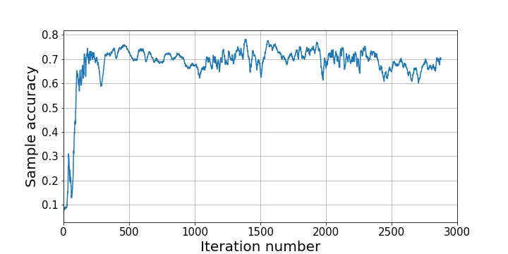
Finally, we can use our built in function hamiltorch.predict_model to evaluate the performance of the samples over the validation.

pred_list, log_prob_list = hamiltorch.predict_model(net, x_val, y_val, samples=params_hmc, model_loss='multi_class', tau_out=1., tau_list=None)
_, pred = torch.max(pred_list, 2)
acc = []
for i in range(pred.shape[0]):
    a = (pred[i].float() == y_val.flatten()).sum().float()/y_val.shape[0]
    acc.append(a)

This results in the following accuracy of samples over iterations:

_{Performance of the samples over the validation set.} _{The expected accuracy over all the samples after iteration 500 is 77.6 %. This is after having only observed 100 digits.}

What’s next for hamiltorch

I am currently writing up my thesis so it might be a while before I implement the next steps but I would like to:

Add additional samplers such as MHMC, NUTS etc…
Add more metrics for RMHMC.

If you have any suggestions feel free to send me an email!

hamiltorch function descriptions

hamiltorch.sample

Parameter	Description
`log_prob_func`	Function handle for a log probability.
`params_init`	Initial value for parameters. Type: PyTorch tensor of shape (D,), where D is the parameter dimension.
`num_samples`	Number of samples. Type: int, Default=10
`num_steps_per_sample`	Number of leapfrog steps (trajectory length). Type: int, Default=10
`step_size`	Step size for numerical integration. Type: float, Default=0.1
`jitter`	Constant multiplier for uniform random variable to be added to diagonal of Fisher. Type: float, Default=None
`normalizing_const`	Normalisation constant for the Fisher (Often equal to size of the data set). Type: float, Default=1.0
`softabs_const`	Controls the softness of the softabs metric. Type: float, Default=None
`explicit_binding_const`	Controls the binding constant for the explicit RMHMC integrator. Type: float, Default=100.
`fixed_point_threshold`	The threshold condition for ending a fixed point loop for the implicit RMHMC integrator. Type: float, Default=1e-5
`fixed_point_max_iterations`	Maximum number of iterations before ending a fixed point loop for the implicit RMHMC integrator. Type: int, Default=1000
`jitter_max_tries`	Maximum number of draws of for jitter, when invalid values for gradients occur. Type: int, Default=10
`sampler`	An instance of the Sampler class that determines the sampler to be used. Type: Sampler object, Default=Sampler.HMC Options: HMC, RMHMC
`integrator`	An instance of the Integrator class that determines the integration scheme to be used. Type: Integration object, Default=Integrator.IMPLICIT Options: EXPLICIT, IMPLICIT
`metric`	An instance of the Metric class that determines the metric to be used. Type: Metric object, Default=Metric.HESSIAN Options: HESSIAN, SOFTABS
`debug`	Debugging flag to print convergence for implicit integration schemes Type: boolean, Default=False

hamiltorch.sample_model

Parameter	Description
`model`	A PyTorch NN model that inherits from the `torch.nn.Module` Type: `torch.nn.Module`
`x`	Input data where the first dimension is the number of data points and the other dimensions correspond to the `model` input shape. Type: `torch Tensor`
`y`	Output data where the first dimension is the number of data points and the other dimensions correspond to the `model` output shape. Type: `Tensor`
`model_loss`	Defines the likelihood for the NN model. Type: string, Default='multi_class' Options: 'binary_class', 'regression'

This is in addition to the same parameters as described for hamiltorch.sample.

First introduced by in Radford M Neal et al. Slice sampling. The annals of statistics, 31(3):705–767, 2003. ↩
As implemented in Michael Betancourt. A general metric for Riemannian manifold Hamiltonian Monte Carlo. In International Conference on Geometric Science of Information, pages 327–334. Springer, 2013. ↩
https://github.com/pytorch/examples/blob/master/mnist/main.py ↩
LeCun, Yann, Bottou, Leon, Bengio, Yoshua, and Haffner, Patrick. Gradient-based learning applied to document recognition. Proceedings of the IEEE, 86(11):2278– 2324, 1998. ↩

Written on July 15th, 2019 by Adam Cobb

Feel free to share!

hamiltorch: a PyTorch Python package for sampling

What is hamiltorch?

Getting started

Sampling a multivariate Gaussian

Simple HMC:

Riemannian HMC:

Sampling from a more complicated distribution

Simple HMC:

Implicit RMHMC:

Explicit RMHMC:

Bayesian neural networks with hamiltorch

What’s next for hamiltorch

hamiltorch function descriptions

You may also enjoy:

Scaling HMC to larger data sets

3D Shape Modelling of Asteroids