Second-Order Optimization without Backpropagation

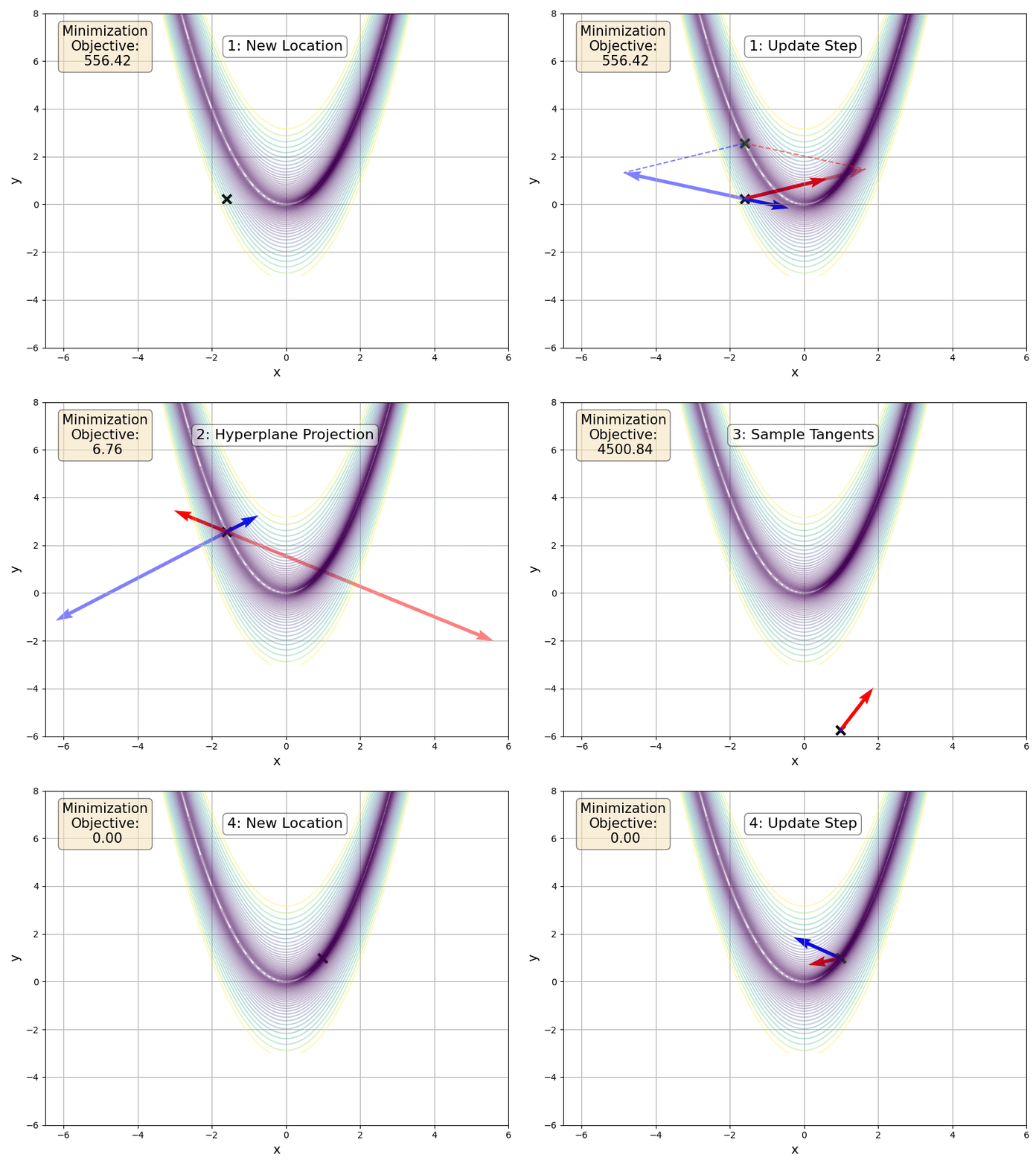
Can we perform optimization without backpropagation? Yes. Recent work by Baydin et al. 2022 has shown that there is promise in using forward-mode automatic differentiation to optimize functions (including neural networks). This is interesting because it removes the need for a backwards pass and opens up the possibility of using energy-efficient hardware for training machine learning models. In recent work, I took this work a bit further by extending to second-order optimization approaches. We will go through this approach and I will demonstrate how to use Fomoh for second-order forward-mode optimization. Further details can be found in “Second-Order Forward-Mode Automatic Differentiation for Optimization”.

Quick links to code blocks:

• FoMoH Hyper-dual Example in Code
• Implementation of FoMoH-2D
• Construction and Comparison of Forward-Mode-Only Optimizers
• Increasing the Dimension of the FoMoH-KD Hyperplane

Background: Forward-Mode and Reverse-Mode Automatic Differentiation

Here, we briefly touch on the two modes of automatic differentiation (AD): Forward-Mode, and Reverse-Mode.

Notation: A bold character, e.g. \(\boldsymbol{\theta}\), denotes a column vector.

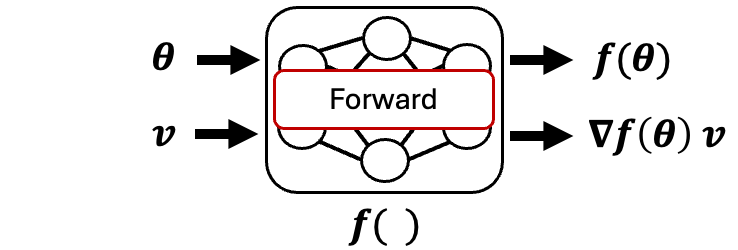Forward-Mode AD

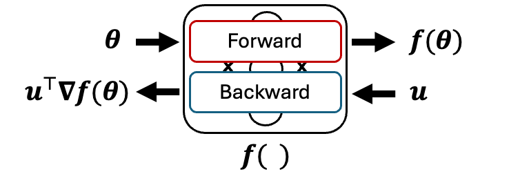Reverse-Mode AD

Forward-Mode AD: \(F(\boldsymbol{\theta}, \mathbf{v})\)

Forward-mode AD applies the chain rule in the forward direction. To gain an intuition of how forward-mode works, we start with a multivariable function with a single output, \(z = f(x,y)\). The first step is to take the total derivative:

We can then set \(\mathbf{v} = [\frac{\mathrm{d}x}{\mathrm{d}t}, \frac{\mathrm{d}y}{\mathrm{d}t} ]^{\top}\), which we will refer to as our tangent vector. To retrieve both partial derivatives, \(\frac{\partial f}{\partial x}\), and \(\frac{\partial f}{\partial y}\), we need to evaluate the total derivative twice, once with \(\mathbf{v} = [1, 0]^{\top}\), and once with \(\mathbf{v} = [0, 1]^{\top}\). We can now generalize this process to a tangent vector \(\mathbf{v}\in\mathbb{R}^D\) and a parameter vector \(\boldsymbol{\theta}\in\mathbb{R}^D\), resulting in a forward-mode procedure \(F(\boldsymbol{\theta}, \mathbf{v})\) that outputs the function evaluation and the corresponding directional derivative at that point (also known as the Jacobian vector product, JVP): \([\boldsymbol{f}(\boldsymbol{\theta}), \nabla \boldsymbol{f}(\boldsymbol{\theta}) \cdot \mathbf{v}]\).

To implement this procedure within an AD framework, one can use dual numbers, where a dual number contains a real (primal) component \(a\in\mathbb{R}\), and a dual component \(b\in\mathbb{R}\). This construction has parallels with imaginary numbers. We can then write out a dual number as \(a + b\epsilon\), and introduce the rule \(\epsilon^2 = 0\). This representation enables us to implement forward-mode AD. For example, if we define the function \(f(a_1 + b_1\epsilon,a_2 + b_2\epsilon)\) as the multiplication of its arguments, then \((a_1 + b_1\epsilon)(a_2 + b_2\epsilon)\) gives us the function evaluation as the primal component and the product rule as the \(\epsilon\) component: \(a_1 a_2 + (a_1 b_2 + a_2 b_1)\epsilon\). We will come back to dual numbers when we meet higher-order forward-mode AD in the next section.

Reverse-Mode AD: \(R(\boldsymbol{\theta}, \mathbf{u})\)

Also known as backpropagation, reverse-mode AD requires a forward pass followed by a reverse pass. The reverse-mode procedure, \(R(\boldsymbol{\theta}, \mathbf{u})\), needs an adjoint vector \(u\in\mathbb{R}^O\), in addition to the parameter vector \(\boldsymbol{\theta}\in\mathbb{R}^D\). For typical optimization problems within machine learning, we are optimizing a single-valued loss function and therefore the adjoint vector can be just set to \(1\). This is implicit in many AD frameworks like PyTorch. The output of the reverse-mode procedure is the function evaluation and the vector-Jacobian product (VJP) \([\boldsymbol{f}(\boldsymbol{\theta}), \mathbf{u}^{\top}\nabla\boldsymbol{f}(\boldsymbol{\theta})]\). We will not explore reverse-mode further in this blog post.

Second-Order Forward-Mode Automatic Differentiation

If we go back to forward-mode automatic differentiation, we can actually extend dual numbers to account for higher-order derivatives. First, let’s write out a dual number in terms of vectors \(\boldsymbol{\theta} + \mathbf{v}\epsilon\). Currently we truncate after the first order (i.e. we set \(\epsilon^2 = 0\)). This results in using dual numbers to represent a first order truncated Taylor series, \(f(\boldsymbol{\theta} + \mathbf{v}\epsilon) = f(\boldsymbol{\theta}) + \nabla f(\boldsymbol{\theta})\cdot \mathbf{v} \epsilon\). To go up one level, we introduce a hyper-dual number \(\boldsymbol{\theta} + \mathbf{v}_1\epsilon_1+ \mathbf{v}_2\epsilon_2+ \mathbf{v}_{12}\epsilon_1 \epsilon_2\), which is made up of four components. This formulation allows us to truncate after the second order by using the definitions \(\epsilon_1^2 = \epsilon_2^2 = (\epsilon_1\epsilon_2)^2 = 0\). This gives our new truncated Taylor series:

What does this mean in practice? It means that a function evaluation with a hyper-dual number gives both first-order and second-order information with one single forward pass. We can actually capture all the elements of the Jacobian and the Hessian of a function by introducing a one-hot basis \(\mathbf{e}_i\) (E.g. \(\mathbf{e}_1 = [1,0,0,...,0], \mathbf{e}_2 = [0,1,0,...,0],...\)) and setting the tangents to these basis vectors, as well as setting \(\mathbf{v}_{12} = \mathbf{0}\). This results in a single forward pass capturing the \(i^{\text{th}}\), and \(j^{\text{th}}\) elements of the Jacobian, as well as the \(ij^{\text{th}}\) element of the Hessian:

Hyper-dual numbers in Fomoh

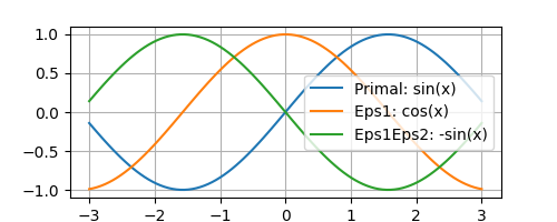
Before going into the details of how we might use forward-mode AD to optimize machine learning models, I will first show how we can use Fomoh to define a hyper-dual number and inspect it. Here, we simply focus on a single-input, single-output \(\sin\) function. We set set \(\mathbf{v}_1\), and \(\mathbf{v}_2\) to ones, as \(\nabla f(\boldsymbol{\theta}) \cdot \mathbf{v}_1 = \frac{\mathrm{d}f}{\mathrm{d}\theta}\) for a single-input, single-output function. Then after passing the hyperdual number x_h through the function, both \(\epsilon_1\) (eps1) and \(\epsilon_2\) (eps2) components correspond to the first derivative, and the \(\epsilon_1\epsilon_2\) (eps1eps2) component corresponds to the second derivative.

from fomoh.hyperdual import HyperTensor as htorch

# Uni-dimensional gives exact outputs:
x = torch.linspace(-3,3,100)
tangent = torch.ones_like(x)

x_h = htorch(x, tangent, tangent)
y_h = x_h.sin() # Forward Pass of hyper-dual tensor

plt.figure()
plt.plot(x_h.real, y_h.real, label = "Primal: sin(x)")
plt.plot(x_h.real, y_h.eps1, label = "Eps1: cos(x)")
plt.plot(x_h.real, y_h.eps1eps2, label = "Eps1Eps2: -sin(x)")
plt.grid()
plt.legend()
plt.show()

Optimization

We now look to see how we can leverage hyper-dual numbers and the Fomoh backend to optimize functions without the use of backpropagation. We will first start with the backpropagation-free approach that leverages first-order information and then move onto our approach that uses second-order information:

Forward Gradient Descent (FGD) ¹ introduced the idea of using forward-mode AD to build estimates (in expectation) of the true gradient. If you sample a tangent vector from a normal distribution, \(\mathbf{v} \sim \mathcal{N}(\mathbf{0},\mathbf{I})\), and multiply the JVP (the dual component of a forward pass), \(\nabla f(\boldsymbol{\theta}) \cdot \mathbf{v}\), by the same tangent vector, this gives the forward gradient: \(\mathbf{g}(\boldsymbol{\theta}) = (\nabla f(\boldsymbol{\theta}) \cdot \mathbf{v}) \mathbf{v}\). Then by leveraging the properties of the Gaussian distribution, where cross terms (\(i\neq j\)) \(\mathbb{E}[v_iv_j] = 0\) and matched terms \(\mathbb{E}[v_iv_i] = 1\), we get \(\mathbb{E}[\mathbf{g}(\boldsymbol{\theta})] = \nabla f(\boldsymbol{\theta})\). As a result, the FGD update rule is given by:

where \(\eta\) is the learning rate. One of the challenges of FGD is that is can be quite sensitive to the learning rate, as well as be susceptible to high variance as the parameters increase in dimension. There are a few papers that focus on this issue ².

Forward-Mode Weight Perturbation with Hessian Information (FoMoH)

Hyper-dual numbers, and the Fomoh backend allow us to extend backpropagation-free optimization to include second-order derivative information. A single forward pass now includes the curvature term in the \(\mathbf{v}\) direction: \(\mathbf{v}^{\top}\nabla^2 f(\boldsymbol{\theta})\mathbf{v}\). This curvature term provides sensitivity information when moving along the tangent directions. For example, when using gradients to optimize a function, taking a gradient step in a region of low curvature is likely to increase the value of the function. However the same sized step in a region of large curvature could significantly change the value of the function (for better or worse). Ideally, we would like to prevent the possibility of “jumping over hills” in the objective function.

To get to our new forward-mode-only update step, we sample a tangent vector from an IID Gaussian (\(\mathbf{v} \sim \mathcal{N}(\mathbf{0},\mathbf{I})\)), and then use the absolute value of the curvature to normalize the directional derivative in the tangent direction. In regions of large curvature, the update step ought to be smaller and therefore enable the update step to move up a hill rather than jumping over it. Therefore the FoMoH update step is:

The directional derivative in the numerator and the curvature (the quadratic form) in the denominator are both provided with one forward-pass of the function \(f(\boldsymbol{\theta}+\mathbf{v}\epsilon_1+\mathbf{v}\epsilon_2+\mathbf{0}\epsilon_1\epsilon_2)\). The normalization via this quadratic form results in accounting for the unit distance at the location \(\boldsymbol{\theta}\) in the direction \(\mathbf{v}\). Therefore, this update step takes into account the distance metric defined at \(\boldsymbol{\theta}\). In regions of high curvature the step size will be smaller, which is a desirable behavior. Like Newton’s method, setting \(\eta \approx 1.0\) seems to work in many cases.

Extending to Forward-Mode Hyperplane Search: FoMoH-KD

One potential challenge of the above FoMoH step, is that the update direction is sampled from a Gaussian distribution and therefore it still relies on the same expectation arguments as FGD. Therefore, we asked: Is there a better way to select a direction while still only relying on forward-mode passes?

Our idea is to build a hyperplane from multiple tangents and then perform a Newton-like step within the hyperplane. We therefore take a more informed update step that we can tradeoff against the cost of a matrix inversion and multiple forward-mode passes. Before going into the details of the algorithm, here is a FoMoH-KD update step operating in 2 dimensions:

FoMoH-KD: The Equations

We build up FoMoH-KD by using \(K=2\) as a running example and then generlize to any \(K\), where the above figure can serve as a visualization. The first step is to sample the two tangent directions, \(\mathbf{v}_1\) and \(\mathbf{v}_2\). Then we evaluate the function of interest, \(f(\cdot)\), with all the hyper-dual tangent pair combinations: \(\{\mathbf{v}_1, \mathbf{v}_1\}\), \(\{\mathbf{v}_1, \mathbf{v}_2\}\), and \(\{\mathbf{v}_2, \mathbf{v}_2\}\). In collecting all these terms, we build the Hessian \(\hat{\mathbf{H}}_{2\times 2}\) in the \(2\times 2\) plane, that we can use to perform a Newton-like step in that hyper-plane. To take such a step, we need to define the step sizes \(\kappa_1\) and \(\kappa_2\) to take in their corresponding tangent directions:

\(\begin{align} \mathbf{\tilde{H}}_{2\times2} &= \left[\begin{array}{cc} \mathbf{v}_1^{\top} \nabla^2 f(\boldsymbol{\theta}) \mathbf{v}_1 & \mathbf{v}_1^{\top} \nabla^2 f(\boldsymbol{\theta}) \mathbf{v}_2 \\ \mathbf{v}_2^{\top} \nabla^2 f(\boldsymbol{\theta}) \mathbf{v}_1 & \mathbf{v}_2^{\top} \nabla^2 f(\boldsymbol{\theta}) \mathbf{v}_2 \end{array}\right], & \left[\begin{array}{c} \kappa_1 \\ \kappa_2 \end{array}\right] &= \mathbf{\tilde{H}}_{2\times2}^{-1} \left[\begin{array}{c} \mathbf{v}_1^{\top} \nabla f(\boldsymbol{\theta}) \\ \mathbf{v}_2^{\top} \nabla f(\boldsymbol{\theta}) \end{array}\right]. \end{align}\) The update step for this 2D example is then:

For a a more general update step in a \(K\)-dimensional hyperplane, we sample \(K\) directions to give:

A manual implementation of FoMoH-2D in Python using Fomoh

Here, I include an implementation of FoMoH-\(K\)D for \(K=2\). In practice, please use the built-in function plane_step_Nd from fomoh.opt as it generalizes to \(K\) dimensions.

from fomoh.hyperdual import HyperTensor as htorch
import torch

def plane_step(fun, x):
    # Sample the two tangent vectors
    v1 = torch.randn(x.shape)
    v2 = torch.randn(x.shape)
    # Stack them for vectorized forward-mode AD
    V1 = torch.cat([v1, v1, v2])
    V2 = torch.cat([v1, v2, v2])
    x_htorch = htorch(x.repeat(3,1), V1, V2)
    # Run the function with the *Fomoh* backend
    z = fun(x_htorch)
    # Build hyperplane Hessian and Hyperplane Jacobian
    H_tilde = torch.tensor([[z.eps1eps2[0], z.eps1eps2[1]],[z.eps1eps2[1], z.eps1eps2[2]]])
    F_tilde = torch.tensor([z.eps1[0], z.eps1[2]]).view(-1,1)
    H_tilde_inv = torch.linalg.inv(H_tilde)
    # Apply Newton-like step to get the steps in the tangent directions
    kappa = - H_tilde_inv @ F_tilde
    # Return update direction
    return kappa[0] * v1 + kappa[1] * v2

Examples in Fomoh library

In an earlier example, we got a flavour of how we can instantiate a hyper-dual number in Fomoh using the HyperTensor class in fomoh.hyperdual, which I will always import as htorch.

2D Rosenbrock Optimization

The Rosenbrock function is a useful test case for non-convex optimization as it contains a known solution that falls in a narrow valley ³:

def rosenbrock(x):
    return (1.-x[:,0]) ** 2. + 100. * (x[:,1] - x[:,0]**2)**2

To optimize this function, we derive a simple update loop that will enable us to change the update step according to our approach of choice:

def optimizer(x_init, fun, update, iterations):
    x = x_init.clone()
    thetas = [x]
    loss = [fun(x).item()]
    for n in range(iterations):
        u = update(x) # minimize
        x = x + u
        loss.append(fun(x).item())
        thetas.append(x.clone())
    return thetas, loss

Using Fomoh, we can define the forward gradient descent update:

def fgd(x, lr = 0.0001):
    v = torch.randn(x.shape)
    z = fun(htorch(x,v,v))
    return - lr * z.eps1 * v

and the FoMoH update:

def fomoh(x):
    v = torch.randn(x.shape)
    z = fun(htorch(x,v,v))
    return - z.eps1 * v / abs(z.eps1eps2)

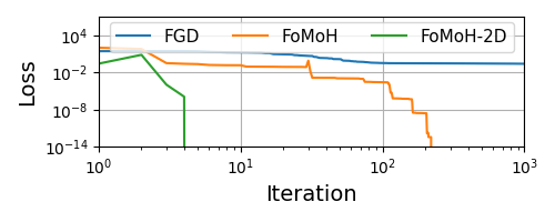
Finally, we just leverage plane_step_Nd to do FoMoH-2D:

from fomoh.opt import plane_step_Nd
fomoh_2d = lambda x: plane_step_Nd(fun, x, 2)

We can then run the optimization routines:

hamiltorch.set_random_seed(0) # Sneaking in hamiltorch

x_init = torch.randn(2).view(1,-1)
fun = rosenbrock
N = 1000 # iterations

## Run optimizers:
fgd_thetas, fgd_loss = optimizer(x_init, fun, fgd, N)
fomoh_thetas, fomoh_loss = optimizer(x_init, fun, fomoh, N)
fomoh_2d_thetas, fomoh_2d_loss = optimizer(x_init, fun, fomoh_2d, N)

FoMoH-KD: increasing the hyperplane dimension

One of the nice characteristics of the Rosenbrock function is that you can extend the function to higher dimensions:

def rosenbrock_ND(x):
    term1 = (1 - x[:, :-1])**2
    term2 = 100 * (x[:, 1:] - x[:, :-1]**2)**2
    return (term1 + term2).sum(-1)

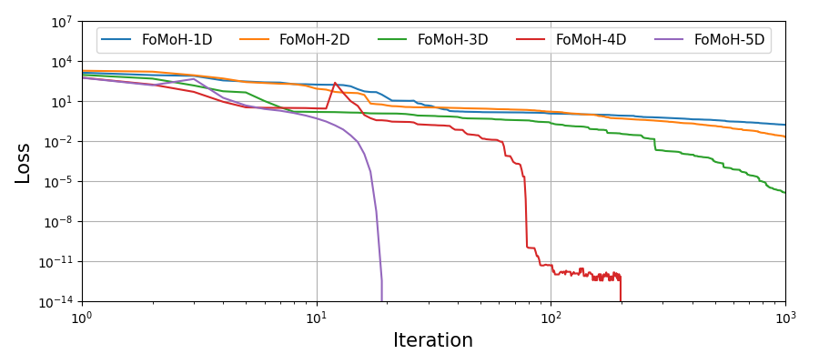
We can now explore how FoMoH-\(K\)D performs as you increase \(K\). To do so, we just iterate the optimizer from \(K=1\) (d in the code) up to \(K=5\). This is for a 5D Rosenbrock function:

hamiltorch.set_random_seed(0)
D = 5 # Dimension of Rosenbrock function
N = 1000 # Optimization Iterations
fun = rosenbrock_ND
x_init = torch.randn(D).view(1,-1)

thetas_list = []
loss_list = []
for d in range(1,D+1):
    # Define K=d update step
    fomoh_Kd = lambda x: plane_step_Nd(fun, x, d)
    ## Run optimizer:
    thetas, loss = optimizer(x_init, fun, fomoh_Kd, N)
    thetas_list.append(thetas)
    loss_list.append(loss)

We can then plot the performance of the optimizers:

Summary

In this blog post I summarized the main points of the paper and provided a short introduction to the Fomoh library. The code in this blog post is included in this notebook. In the next blog post, I will focus on training neural networks, and how the Fomoh code base mimics PyTorch.

Acknowledgements

This material is based upon work supported by the United States Air Force and DARPA under Contract No. FA8750-23-C-0519. Any opinions, findings and conclusions or recommendations expressed in this material are those of the author(s) and do not necessarily reflect the views of the United States Air Force and DARPA.