Scaling HMC to larger data sets

In this blog post I will demonstrate how to use hamiltorch for inference in Bayesian neural networks with larger data sets. Further details can be found in “Scaling Hamiltonian Monte Carlo Inference for Bayesian Neural Networks with Symmetric Splitting”.

hamiltorch for Bayesian neural networks

Towards the end of my previous post I gave a basic example of how to use hamiltorch for inference in Bayesian neural networks (BNNs). Since then, my aim has been to make it as easy as possible to apply HMC over as many PyTorch models as possible. This includes being able to work with a torch.utils.data.Dataloader in the same way as for stochastic gradient descent. However, the main addition since the last post, has been to investigate split HMC and come up with a new way of scaling HMC to larger data sets with a single GPU. Interestingly, we will actually see that hamiltorch can compete with stochastic gradient approaches and also provide better uncertainty quantification.

Regression

As a reminder of how to use hamiltorch, we will start with a simple regression task. We will use a data set¹ that nicely tests how models behave outside the range of the data. Here, we will focus on the main highlights and leave details such as data loading and pre-processing to the full notebook. In addition, some details are left to the previous tutorial notebooks.

Let’s first define our fully-connected neural network in PyTorch:

import torch.nn as nn
import torch.nn.functional as F
class Net(nn.Module):
    def __init__(self):
        super(Net, self).__init__()
        self.fc1 = nn.Linear(1, 100)
        self.fc2 = nn.Linear(100, 100)
        self.fc3 = nn.Linear(100, 1)

    def forward(self, x):
        x = F.relu(self.fc1(x))
        x = F.relu(self.fc2(x))
        x = self.fc3(x)
        return x
net = Net()

Now, as we are working with a regression task we will be using a Gaussian likelihood,

(i.e. the squared error). The network, \(\mathbf{f}_{\mathrm{net}}(\mathbf{X};\boldsymbol{\omega})\), is a function of the input, \(\mathbf{X}\), and the weights, \(\boldsymbol{\omega}.\) Therefore, all that remains to be defined for the likelihood is the output precision, \(\tau_{\mathrm{out}}\), or the parameter tau_out. For now, we will infer it via Gaussian process regression to get tau_out = 110.4, however this output precision is a hyperparameter that can otherwise be found from cross-validation.

The final component specific to inference with BNNs is setting the prior. We currently use a simple layer-wise Gaussian prior over the weights, where the covariance of each layer is only defined by the diagonal scaling factor \(\tau_l\), where

Therefore, as we have 3 linear layers with a set of weights and biases per layer, we must set 6 prior precisions. Here, we simply set them via the parameter, tau_list = torch.tensor([1., 1., 1., 1., 1., 1.], device='cuda:0'). This corresponds to a simple \(\mathcal{N}(\mathbf{0},\mathbf{I})\) prior.

We are now ready to run a simple HMC inference

Simple HMC:

step_size = 0.0005
num_samples = 1000
L = 30 # Remember, this is the trajectory length
burn = -1
store_on_GPU = False # This tells sampler whether to store all samples on the GPU
debug = False # This is useful for debugging if we want to print the Hamiltonian
model_loss = 'regression'
tau = torch.tensor([1., 1., 1., 1., 1., 1.], device=device)
tau_out = 110.4
mass = 1.0 # Mass matrix diagonal scale
params_init = hamiltorch.util.flatten(net).to(device).clone()
inv_mass = torch.ones(params_init.shape) / mass # Diagonal of inverse mass matrix

print(params_init.shape)
integrator = hamiltorch.Integrator.EXPLICIT
sampler = hamiltorch.Sampler.HMC # We are doing simple HMC with a standard leapfrog

hamiltorch.set_random_seed(0)
# Let's sample!
params_hmc_f = hamiltorch.sample_model(net, X.to(device), Y.to(device), params_init=params_init,
                                       model_loss=model_loss, num_samples=num_samples,
                                       burn = burn, inv_mass=inv_mass.to(device), step_size=step_size,
                                       num_steps_per_sample=L ,tau_out=tau_out, tau_list=tau_list,
                                       store_on_GPU=store_on_GPU, sampler = sampler)
# Let's move the final sample of each trajectory onto the GPU for later
params_hmc_gpu = [ll.to(device) for ll in params_hmc_f[1:]] # We remove the first sample (params_init)

Output:

torch.Size([10401])
Sampling (Sampler.HMC; Integrator.IMPLICIT)
Time spent  | Time remain.| Progress             | Samples   | Samples/sec
0d:00:01:19 | 0d:00:00:00 | #################### | 1000/1000 | 12.62       
Acceptance Rate 0.59

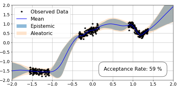
OK, so that was a lot of code without much of an explanation. However, if we break it down, it should make more sense. At the start, we initialise the step-size and trajectory length of the sampler, as well as the number of samples. We decide to burn none of the samples for now, and save space on the GPU by moving all the samples to the CPU. We set the loss to regression. We then set our mass matrix for HMC. Finally, we pass all these arguments into hamiltorch.sample_model (as before) and run the code. We then move the accepted samples at the end of each trajectory to the GPU for analysis.

For now, we are passing in torch tensors X and Y as training data and we are going to evaluate our samples over the test set X_test = torch.linspace(-2,2,500).view(-1,1):

predictions, log_probs_f = hamiltorch.predict_model(net, x = X_test.to(device),
                                                  y = X_test.to(device), samples=params_hmc_gpu,
                                                  model_loss=model_loss, tau_out=tau_out,
                                                  tau_list=tau_list)

We have now completed the pipeline for full HMC and we can plot the results.

Scaling to larger data sets with symmetric split HMC

One of the limitations of working with HMC is that we need to work with a data set that we can fit into GPU memory (in its entirety). In recent work, I have been looking at ways to overcome this challenge by using splitting. This is not a new idea, however our motivation is different to before with the aim of scaling HMC to larger data sets. The simple idea is to allocate the data into small subsamples and then compute the entire Hamiltonian by shuffling the subsamples on and off the GPU. Of course, the computational complexity of this approach is heavily dependent on the size of the GPU memory and the size of the data, but this method will allow us to use a single GPU to perform HMC whilst avoiding any bias associated with stochastic batches.²

Let’s stick with the regression example and sample with the hamiltorch function for split HMC, hamiltorch.sample_split_model.

First, we can now work with PyTorch data loaders, which are much more convenient. Therefore, we can define these via the code:

batch_size = 100
data_tr = RegressionData(X, Y)
data_val = RegressionData(X_test, X_test) # I have implicitly set Y_test = X_test as we have no ground truth so it is just as a dummy array.

dataloader_tr = DataLoader(data_tr, batch_size=batch_size,
                        shuffle=True, num_workers=4)
dataloader_val = DataLoader(data_val, batch_size=len(X_test),
                        shuffle=False, num_workers=4)

This gives us a training and validation data set and corresponding data loaders. We then follow almost the same structure as before, except we use the sampler for splitting and we set integrator = hamiltorch.Integrator.SPLITTING:

M = X.shape[0] / batch_size # Number of subgradient splits

print(params_init.shape)
integrator = hamiltorch.Integrator.SPLITTING # Here we select the default splitting scheme
sampler = hamiltorch.Sampler.HMC

hamiltorch.set_random_seed(0)
# Note the second parameter is now dataLoader_tr
params_hmc_s = hamiltorch.sample_split_model(net, dataloader_tr, params_init=params_init,
                                             num_splits=M, num_samples=num_samples,
                                             step_size=step_size, num_steps_per_sample=L,
                                             inv_mass = inv_mass.to(device), integrator=integrator,
                                             debug = debug, store_on_GPU=store_on_GPU, burn = burn,
                                             sampler = sampler, tau_out=tau_out, tau_list=tau_list, model_loss=model_loss)

params_hmc_gpu = [ll.to(device) for ll in params_hmc_s[1:]]

Output:

torch.Size([10401])
Number of splits:  4  , each of batch size  100

Sampling (Sampler.HMC; Integrator.SPLITTING)
Time spent  | Time remain.| Progress             | Samples   | Samples/sec
0d:00:10:10 | 0d:00:00:00 | #################### | 1000/1000 | 1.64       
Acceptance Rate 0.93

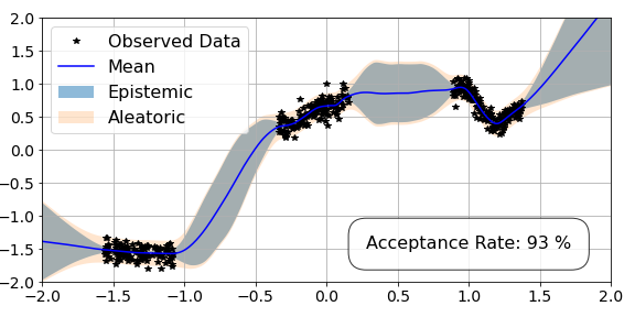
We also have a new argument called num_splits. This corresponds to the number of data subsets that we will perform novel symmetric split HMC over, which is 4 in this case (4 splits each of 100). In the output box, we see both the advantage and disadvantage of this approach. The disadvantage is that it is slower, as we have to move data on and off the GPU. However the advantage is the efficiency of the sampler as it has a much higher acceptance rate for the same hyperparameters. In fact, we show in our paper that this efficiency is a very useful property.

Now, as before we can use the predict_model function but we can simply pass the validation data loader directly:

predictions, log_probs_s = hamiltorch.predict_model(net, test_loader = dataloader_val,
                                                    samples=params_hmc_gpu,
                                                    model_loss=model_loss, tau_out=tau_out,
                                                    tau_list=tau_list)

We can then plot our results for novel symmetric split HMC below.

Uncertainty quantification with novel symmetric split HMC

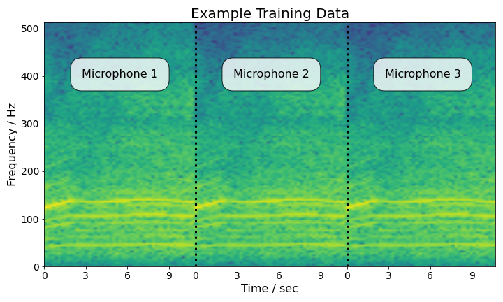
We now move on to a more challenging example to demonstrate the advantages of this new splitting approach for a larger data set. Therefore, we will now take the vehicle classification example from the paper and take a close look at the uncertainty quantification.³

We will also compare to stochastic gradient Markov chain Monte Carlo (MCMC) approaches, as they are the main MCMC competitor for scaling BNN inference. Therefore, we will include stochastic gradient Langevin dynamics (SGLD)⁴ and stochastic gradient HMC (SGHMC)⁵. Also, for a deterministic comparison, we will also include stochastic gradient descent (SGD).

Unlike the regression example, we can no longer fit the entire data set onto the GPU and compute the gradient of the full Hamiltonian. Therefore, we will be using novel symmetric split HMC as we did above. The data set consists of acoustic readings for 9 classes of vehicles. After pre-processing, the input data to the model looks as follows:

At this point, we will follow the same approach as for the regression example and run novel symmetric split HMC over the data set (please refer to the paper for more details). We also run the baselines.

How do we go about analysing uncertainty?

There are multiple ways to analyse the results. Having run the code, we now have a collection of model weights (i.e. \(\{\boldsymbol{\omega}\}_{s=1}^{S}\)) for each Monte Carlo inference scheme and a single model for SGD. We want the output of our model to display its confidence in a label. For example, for 9 classes, the least confident prediction would be a vector of [1/9, 1/9, 1/9, 1/9, 1/9, 1/9, 1/9, 1/9, 1/9]. This vector corresponds to the maximum entropy prediction, which indicates a high level of uncertainty. On the other hand, a minimum entropy prediction would look like a vector of [1, 0, 0, 0, 0, 0, 0, 0, 0], which corresponds to the highest confidence possible. For this case, we better hope that the model is correct, because with 100 % confidence we would not be in a position to suspect any chance of an error.

Therefore, the predictive entropy is a good way to navigate from the softmax output to a single value that can indicate the confidence of a model in its prediction. For SGD this is simply \(- \sum_c p_c \log p_c\) for a single test input \(\mathbf{x}^*\), where \(p_c\) corresponds probability of each class (i.e. each element in the vector). For the Monte Carlo approaches there are multiple outputs, where each output corresponds to a different weight sample, \(\boldsymbol{\omega}^{(s)}\). There are different ways to work with the entropy formulation, but we start with the standard solution which is to average over the outputs and then work with the expected value of the output. This corresponds to the posterior predictive entropy, \(\tilde{\mathcal{H}}\):

Of course, this does not take into account the origin of the uncertainty (i.e. is it the model that is unsure, or is the data simply noisy), but for practical purposes it is a useful tool as it will tell us how much to trust the prediction.

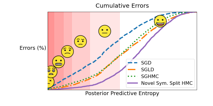
Using \(\tilde{\mathcal{H}}\), we can start to look at the uncertainty behaviour of the models. In particular, it is helpful to look at the errors and see if they were made in a catastrophic manner. One way to do this is to plot the cumulative sum of \(\tilde{\mathcal{H}}\) for all the mistakes made by the models. This plot can tell us what proportion of the erroneous predictions were made with high confidence. Let’s look at the plot:

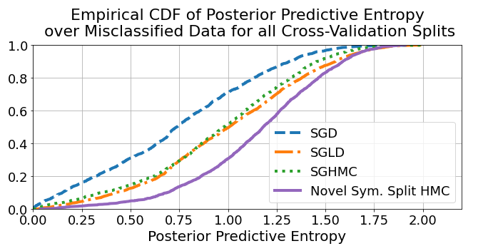
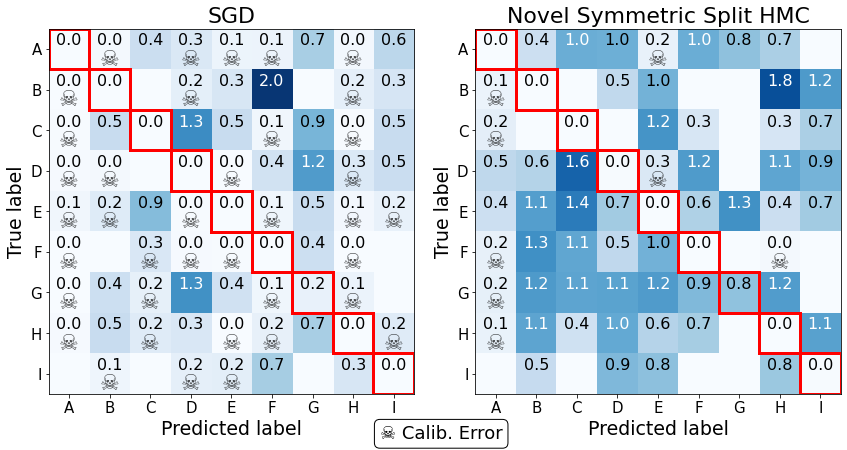
Although the above graph informs us about the distribution of errors, it is also useful to look at a per class performance. While there are multiple ways of representing uncertainty performance, we can look at the worst-case scenario in a “confusion-style” matrix. That is, we can take the minimum value of the predictive entropy that falls in each square and see whether these minimum entropy predictions lead to catastrophic performance.

We compare the worst performing model, SGD, with the best, novel symmetric split HMC. To help highlight the “dangerous performance”, off-diagonal squares with data \(\mathcal{H} < 0.3\) are highlighted with “☠️”. This loosely translates to a scenario where the softmax probability of a wrong class is 0.95 with the rest being equal (although in reality there are multiple mappings).

Further uncertainty decomposition: the mutual information

Finally, there are other ways that we can decompose the uncertainty to identify the model uncertainty from the data uncertainty.⁶ Why would we want to do this? Well, it might be helpful to distinguish between two scenarios that \(\tilde{\mathcal{H}}\) cannot capture:

• A scenario where all samples are equally uncertain.
• A scenario where all samples are certain, yet completely disagree.

For example, it might be the case that all the Monte Carlo samples for the same input result in multiple predictions, with all having the same exact maximum entropy distribution, [1/9, ... , 1/9]. The \(\tilde{\mathcal{H}}\) resulting from this scenario would, however, be the same as sampling 9 Monte Carlo predictions, where each prediction assigns a 1.0 to a different class. To distinguish between the two cases, we first introduce the expectation over the entropy with respect to the parameters:⁷

Now, if we go back to our example of predictive samples consisting of one-hot vectors (e.g. nine different [1, 0, 0, 0, 0, 0, 0, 0, 0]), then \(\mathbb{E} [\mathcal{H}] = 0\), however \(\tilde{\mathcal{H}} \neq 0\) (and would in fact be at its maximum value of 2.20 if all the 9 one-hot vectors were unique). This now allows us to determine whether the uncertainty in our model is due to high disagreement between samples, which could be due to an out of distribution test point, or whether the model is familiar with the data regime but is uncertain as it “recognises” the noise.

The mutual information between the prediction \(\mathbf{y}^*\) and the model posterior over \(\boldsymbol{\omega}\) can then be written as:

The mutual information (MI) will measure how much one variable, say \(\boldsymbol{\omega}\), tells us about the other random variable, say \(\mathbf{y}^*\) (or vice-versa). If \(I(\mathbf{y}^* ,\boldsymbol{\omega}) = 0\), then that tells us that \(\boldsymbol{\omega}\) and \(\mathbf{y}^*\) are independent, given the data. One way to think about this, is to consider the scenario where the predictions completely disagree with each other for a given \(\mathbf{x}^*\). In this case, for each \(\boldsymbol{\omega}_s\) drawn from the posterior, we get very different predictions. This informs us that the \(\mathbf{y}^*\) is very dependent on the posterior draw and thus \(I(\mathbf{y}^* ,\boldsymbol{\omega}) \gg 0\) (as \(\tilde{\mathcal{H}} \gg \mathbb{E} [\mathcal{H}]\)). However, if \(\mathbf{y}^* =\) [1/9, ... , 1/9] for all \(\boldsymbol{\omega}_s \sim p(\boldsymbol{\omega}\vert \mathbf{Y,X})\), then the different draws from the posterior distribution have no effect on the predictive distribution and therefore the mutual information between the two distributions is zero (they are independent).⁸

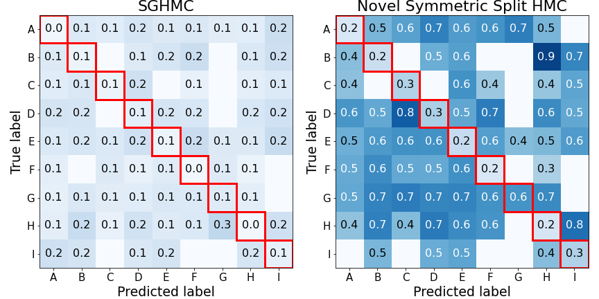
Now, we have the general idea of what the mutual information is, we can go back to the case study. Once again, we can look at the “confusion-style” matrices but for the mutual information. This time, each square corresponds to the average \(I(\mathbf{y}^* ,\boldsymbol{\omega})\), where the average is taken with respect to the number of data points falling in each square.

What’s next for hamiltorch

There’s a lot more to do! Please feel free to send me an email if you have any suggestions, I have received many already and it is very helpful for making improvements!

Of course, if you are interested in looking at the code, please visit the github repo.

Acknowledgements

hamiltorch is a project that I continue to work on while I do research. Therefore its development has benefitted from input from multiple people, including contributions from the GitHub community. The work in this particular post (and corresponding paper) was made possible due to the great supervision of Dr Brian Jalaian!

We would like to thank Tien Pham for making the data available and Ivan Kiskin for his great feedback. ACIDS (Acoustic-seismic Classification Identification Data Set) is an ideal data set for developing and training acoustic classification and identification algorithms. ACIDS along with other data sets can be obtained online through the Automated Online Data Repository (AODR).⁹ Research reported in this paper was sponsored in part by the CCDC Army Research Laboratory. The views and conclusions contained in this document are those of the authors and should not be interpreted as representing the official policies, either expressed or implied, of the Army Research Laboratory or the U.S. Government. The U.S. Government is authorized to reproduce and distribute reprints for Government purposes notwithstanding any copyright notation herein.