Do Diffusion Models Dream of Electric Planes?

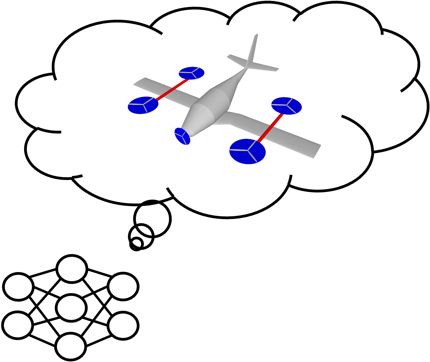
Have you ever wondered what it might be like to let diffusion models go rogue and come up with crazy aircraft designs? Well, now is your chance to see what happens. In this blog post I summarize our recent paper: “Do Diffusion Models Dream of Electric Planes?” Discrete and Continuous Simulation-Based Inference for Aircraft Design.¹

Motivation

Conceptual aircraft design is a slow iterative process and requires multiple rounds of simulation. At this early stage of design, tools must be flexible and fast. Initially, we might not even know how many wings we want (or need) given some specification.

However, designers will have a goal in mind. For example, their high-level goal might be: “I need an eVTOL that can pick people up at LAX airport and drop them off at the Olympic Park.” This goal is then translated into specific design requirements such as “the amount of charge needed for a single trip” or maybe even “lift and drag coefficients.” The next stage of the process is a bit more arduous. Designers need to come up with the aircraft that achieve these goals. In some instances, the specification is on the input, such as a wingspan limit. However, in other instances, the specification is on the output, such as the coefficient of lift and drag (where we only know these values after simulation). Inverse design means starting from the outputs and inferring the inputs. In reality, designers require a tool that enables conditioning on both inputs and outputs.

For designers, a tool that is flexible and fast might enable exploring deisgns that lie outside traditional “design silos.” Machine learning can therefore play an important role at this exploratory stage. We arrive at our goal:

---

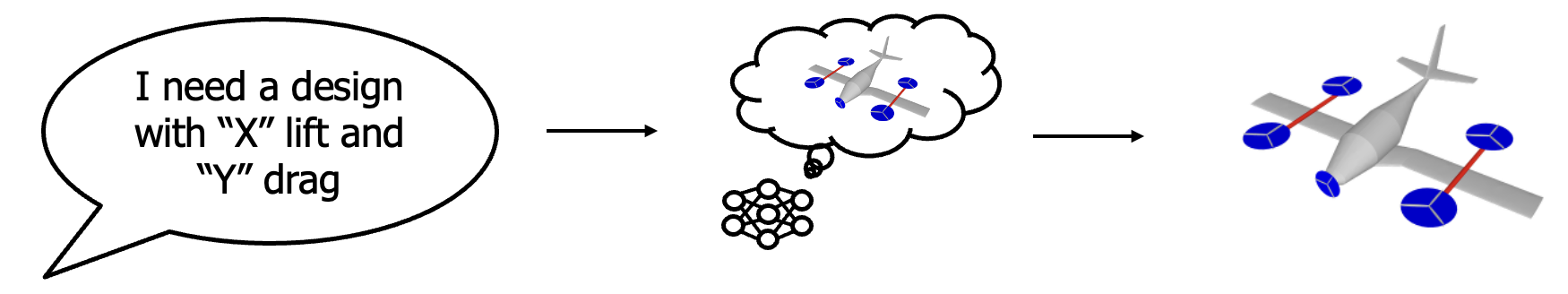
_{Inverse design starts with desired performance metrics and is well-matched to a designer's thought process.}

---

Simulation-based inference as inverse design

Traditional tools that simulate aircraft operate in the “forward direction”. One takes a design, passes it through a simulator and observes the outputs. This forward evaluation of the system may also be non-deterministic. For example, an aircraft may run the same mission with different weather settings, or the simulator may add sensor noise to the aircraft. Let’s call one forward evaluation from the simulator a sample from a likelihood, $\mathbf{x} \sim p(\mathbf{x} \mid \boldsymbol{\theta})$, where $\mathbf{x}$ is our observation conditioned on the design parameters, $\boldsymbol{\theta}$. I illustrate this data generating process below.

---

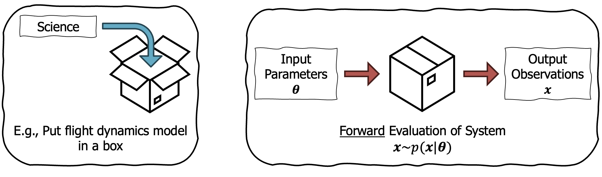
_{We can sample from the forward model to generate data.}

---

Note, that while we can generate data by sampling from this likelihood, we do not know its analytical form. This is in contrast to scenarios where we define a Gaussian likelihood or a categorical likelihood.²

Since our aim is inverse design, we want to invert this simulator and model the posterior, $p(\boldsymbol{\theta}\mid \mathbf{x})$. Then we would have the ability to sample designs conditioned on the desired simulator outputs. This is where we arrive at Simulation-Based Inference (SBI)³.

SBI tackles the problem of inverting stochastic simulators when one does not have access to the analytical form of the likelihood.

Essentially, we want to perform Bayes’ rule,

\[\color{#000000}{p(\boldsymbol{\theta}\mid \mathbf{x})} = \frac{\color{#c65a5a}{p(\mathbf{x}\mid \boldsymbol{\theta})}\,\color{#000000}{p(\boldsymbol{\theta})}}{\color{#000000}{p(\mathbf{x})}},\]

where red denotes the missing likelihood. While most approaches in Bayesian inference target scenarios without knowing the evidence (denominator), SBI has the additional challenge of working without the likelihood.

---

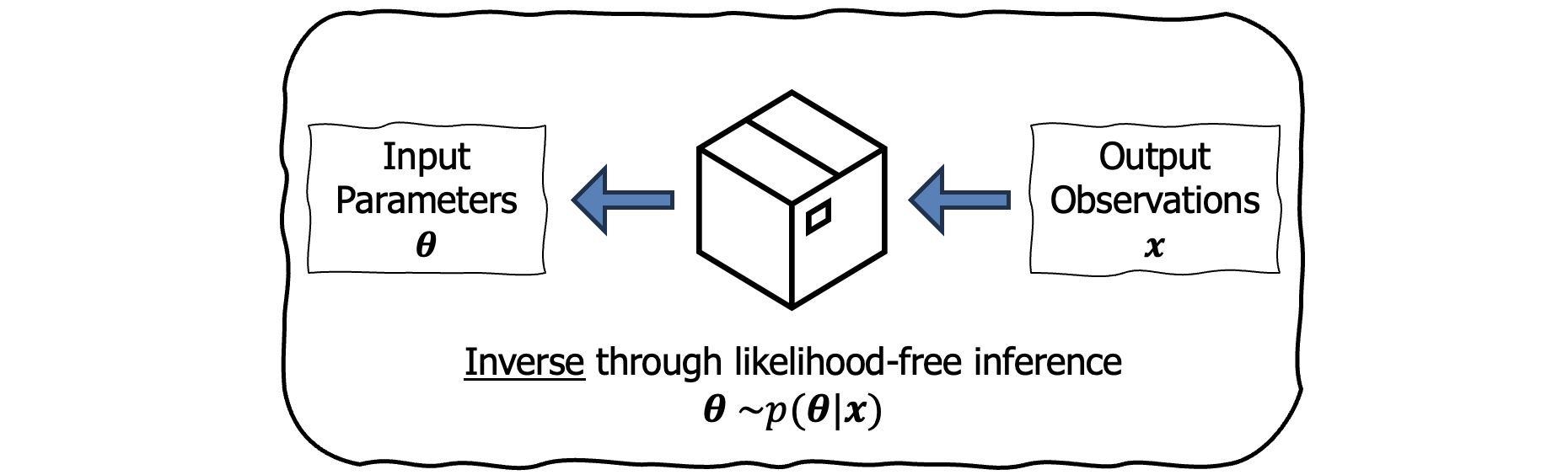
_{SBI learns the inverse model to enable conditioning on the output of a simulation.}

---

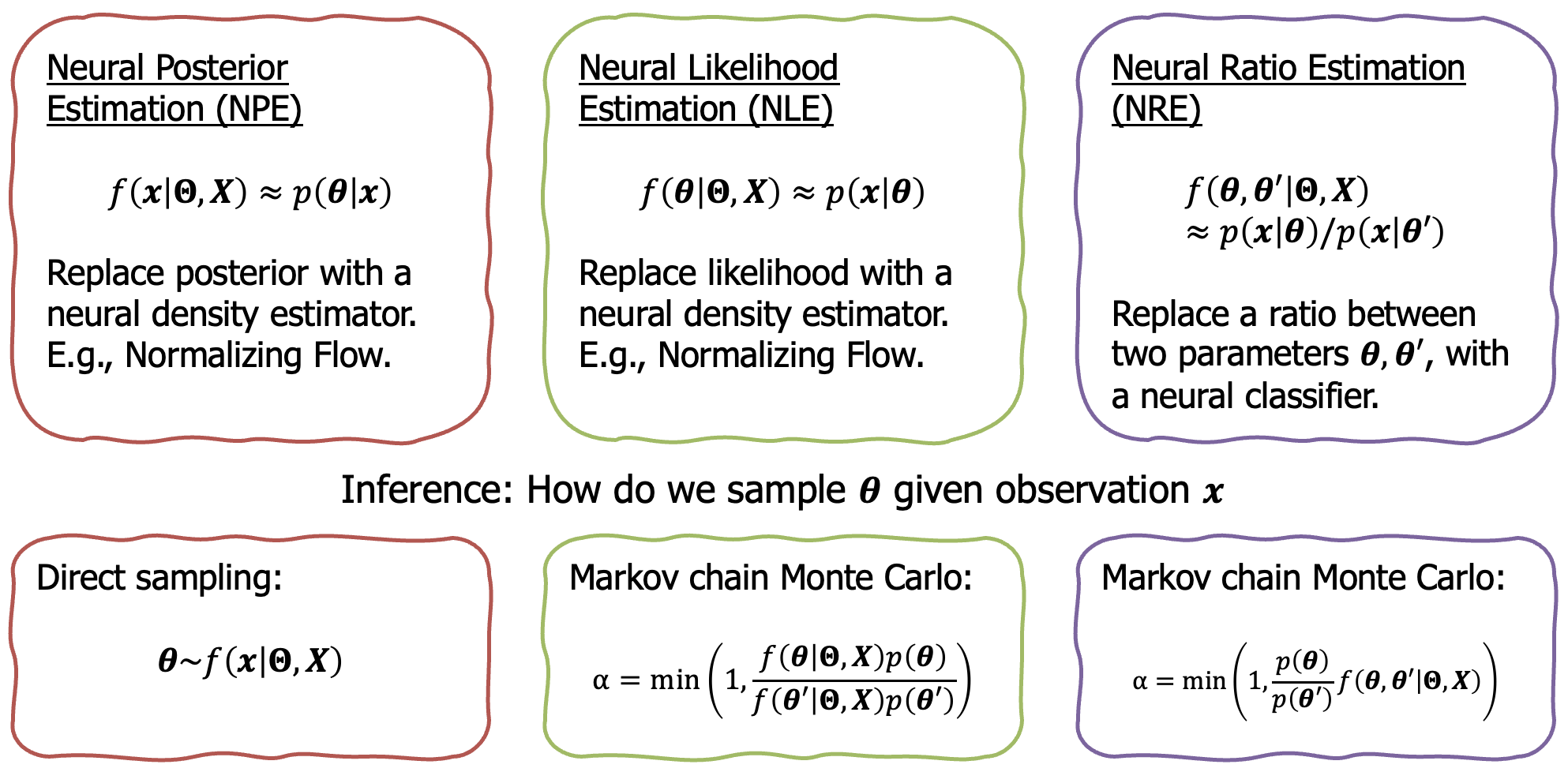
Existing SBI approaches include neural likelihood estimation, neural posterior estimation, and neural ratio estimation. See below.

---

---

However, a recent approach by Gloeckler et al. (2024) introduced the flexibility and scalability of using diffusion models for SBI. ⁴ Rather than targeting a specific component of Bayes’ rule, the diffusion model learns the joint distribution, $p(\boldsymbol{\theta}, \mathbf{x})$. Then, one can generate “missing” parameters, conditioned on “fixed” parameters. For example, fixing $\mathbf{x}$ and sampling $\boldsymbol{\theta}$, means sampling from the posterior. A similar reasoning is used for the likelihood as well, but with the parameters and observations switched. However, even more interesting is the ability to fix subsets of both the parameters and observations. Hence, why diffusion models might be flexible enough for design!

Aircraft design

While we found diffusion models to be appealing for aircraft design, they did not solve two key challenges:

1. Aircraft design consists of discrete and continuous parameters.
2. The dimensionality of the parameters changes depending on the number of components. For example, a design with two wings requires an extra set of wing parameters compared to a design with one wing.

Thinking about these challenges practically, we can see the problem. Imagine trying to run a diffusion model to generate an artifact. What happens if halfway through the denoising process, it veers from a design with one wing to a design with two wings? The number of parameters would change, and the support for the diffusion process would change as well, which is not something easily dealt with.⁵

To tackle this problem, we need to introduce some notation. We define an aircraft design via its topology $\boldsymbol{\tau}$, and parameters, $\boldsymbol{\theta}$. $\boldsymbol{\tau}$ determines the number of components of a design (aircraft configurations). This includes determining the number of wings, the number of propellers etc. Depending on the topology, the parameters, $\boldsymbol{\theta}\in\mathbb{R}^{D_{\boldsymbol{\tau}}}$, will have a different size, $D_{\boldsymbol{\tau}}$. Finally, we continue to use $\mathbf{x}$ as the observation from the simulator. As a result, a design is fully defined by $\{\boldsymbol{\theta} ,\boldsymbol{\tau}\}$.

In this blog post we will refine the goal, and focus posterior sampling:⁶

Remembering the two key challenges from above, sampling from this joint is hard. Therefore the first key insight in our work is to split the posterior into a hierarchical model:

At this stage, we can offer a TLDR:

MixeDiT-MaskeDiT architecture

Hopefully by this point we are sufficiently motivated to tackle the technical part of the work. We will start with the Mixed Diffusion Transformer (MixeDiT), followed by the Masked Diffusion Transformer (MaskeDiT).

---

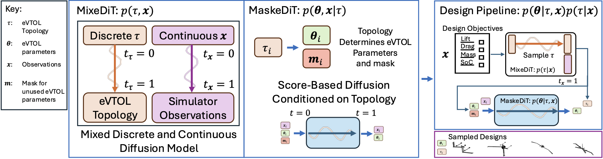
_{Overview figure highlighting: the MixeDiT model on the left that facilitates discrete and continuous sampling; the MaskeDiT model in the middle that samples the parameters conditioned on the topology; and the right shows the procedure for sampling from the posterior $p(\boldsymbol{\theta} \mid \boldsymbol{\tau}, \mathbf{x})p(\boldsymbol{\tau} \mid \mathbf{x})$.}

---

Discrete and continuous sampling with MixeDiT

Since I started working on using machine learning for designing cyber-physical systems, there has always been this challenge in sampling discrete and continuous parameters.⁷ While the approach I am about to describe is likely not the only way, it seems to solve a lot of the challenges.

I had to read two separate papers before arriving at this approach:

1. The first was a really nice paper highlighted at the end of the MIT course on Flow Matching and Diffusion Models. The paper by Zhu et al. (2025) ⁸ introduces “Unified World Models”, which couples two independent continuous diffusion processes into the same model. In their example, they coupled predicted observations and actions. The flexibility of this approach means one can sample from the joint distribution using the coupled diffusion process. Furthermore, fixing the time, $t=1$, for one of the inputs is the equivalent to conditioning on that input. We will explore this in a bit.
2. When going through all the diffusion model papers at NeurIPS 2025 I came across a really cool paper by Jo & Hwang (2025)⁹. They introduce the Riemannian Diffusion Language Model (RDLM), which is a continuous diffusion approach to language modeling. Their insight is to take the one-hot representation of a token, convert to the continuous probability simplex, and then use a known diffeomorphism to transform to the positive orphant of a hypersphere (which comes with its own Riemannian metric to measure distance). The details of the paper are really interesting, but in short, this means we can now run a continuous diffusion model and then transform back into the discrete space at the end.

MixeDiT. The above two papers enable the coupling of two diffusion processes and for one of those processes to correspond to a discrete variable. Specifically, during the reverse process of the diffusion model, the coupled diffusion process operates in the continuous space. At the end, the discrete component is transformed back into the discrete space. As such, we arrive at a model that can sample a mixture of discrete and continuous parameters. Or, in the case of aircraft design, we can jointly sample a topology and an observation.

Since this is a blog post, we will focus on the conceptual understanding, and specifically the more natural inverse-design scenario of sampling a topology (or aircraft configuration) conditioned on a desired output performance, $p(\boldsymbol{\tau} \mid \mathbf{x})$. Think of this stage as, once we have a learned the MixeDiT model, we use it to sample the most likely topologies conditioned on a desired performance. We will see, for example, that conditioning on a lower mass design means fewer sampled topologies with a second wing.

---

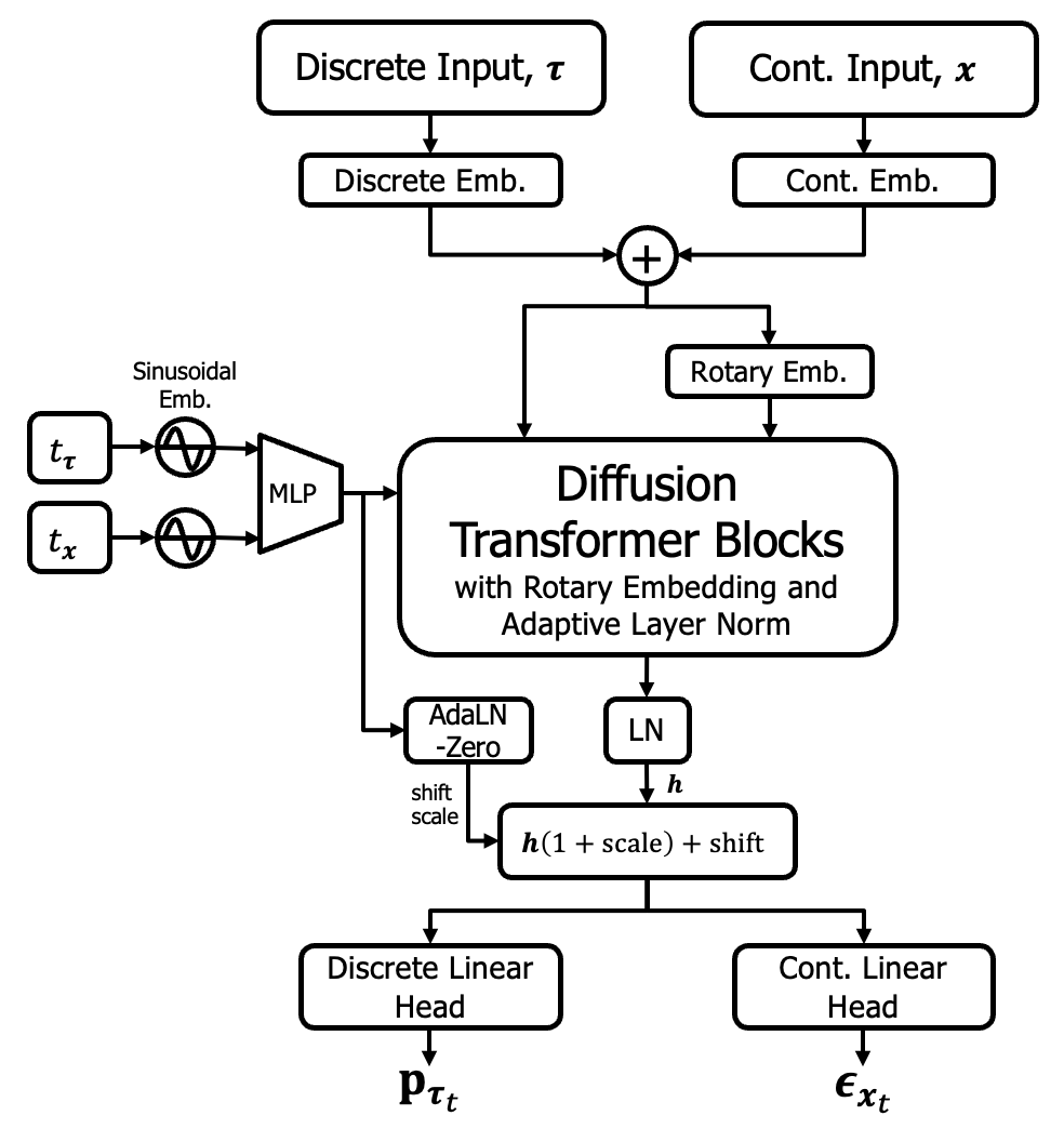
_{MixeDiT: Enables discrete and continuous sampling. The dual input and output, with the independent timesteps for the aircraft topology and observation, results in the flexibility to condition on the observation and sample the topology i.e. $p(\boldsymbol{\tau} \mid \mathbf{x})$ by fixing $t_{\mathbf{x}}=1$, or vice-versa $p(\mathbf{x} \mid \boldsymbol{\tau})$ by fixing $t_{\boldsymbol{\tau}}=1$.}

---

When referring back to our “Extra Refined Goal,” we have now learnt the first level of the hierarchy, $p(\boldsymbol{\tau} \mid \mathbf{x})$, corresponding to MixeDiT.

Sampling designs of varying lengths with MaskeDiT

By this stage of the hierarchy, we have settled on a topology. Therefore, the challenge is to build a model that can condition on any topology, with the important caveat being that different topologies lead to a different parameter dimensions. The solution is to use the approach of masking in transformer-based models, such that the topology prescribes which parameters are masked out and do not contribute to the attention mechanism. Unlike in the Simformer⁴ paper, we use a noise-matching loss as we found it to provide more stable performance.

---

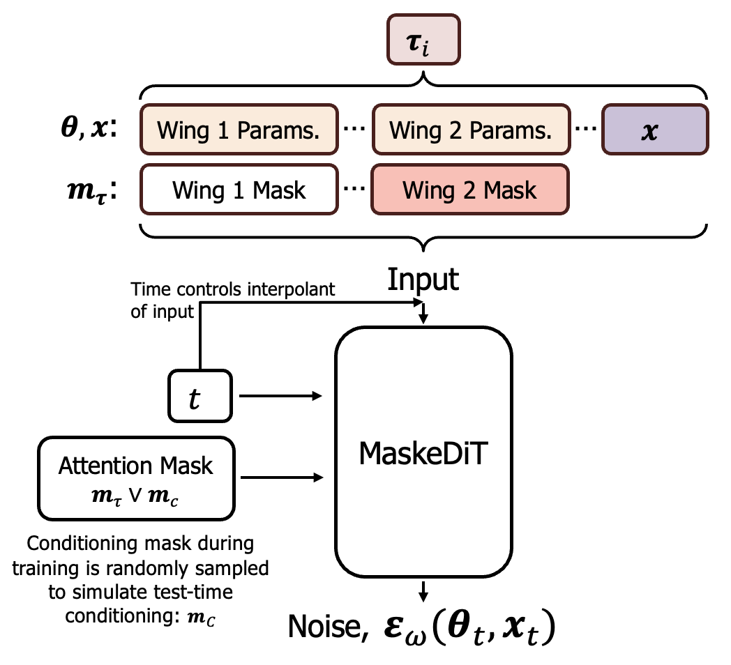
_{MaskeDiT: The aircraft topology controls the masking of certain parameters. In this example the topology does not have a second wing, so the parameters such as wing span and chord length corresponding to the second wing are masked out. The conditioning mask carries over from the original Simformer paper, the topology mask ensures that unused parameters do not influence the diffusion process.}

---

Let’s evaluate the aircraft design pipeline

In the paper, we show a few different ways of evaluating the performance of the MixeDiT-MaskeDit architecture. Here, we will start with the “completion of the loop”, or the Posterior Predictive Check (PPC).

---

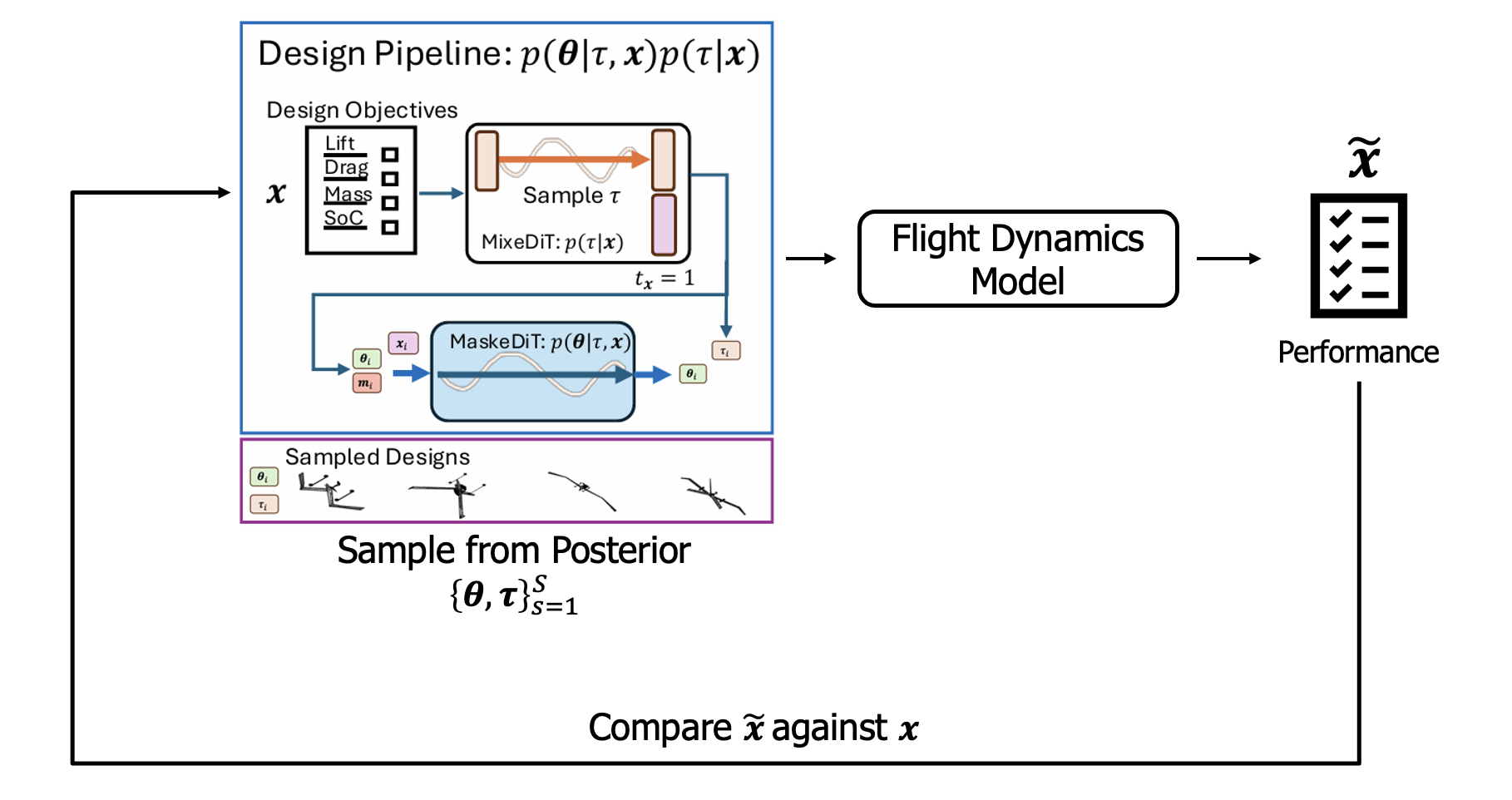
_{Posterior Predictive Check: To evaluate our inverse design pipeline, we condition on design metrics $\mathbf{x}$, run the MixeDiT-MaskeDiT design pipeline to get a design, $\{\boldsymbol{\theta},\boldsymbol{\tau}\}$, then run that design through the original simulator and compare the simulation performance metrics $\tilde{\mathbf{x}}$ with the original design objective.}

---

We now show an example of one of these PPCs, where red corresponds to the design objective, and the dashed line is the mean of the posterior sample:

---

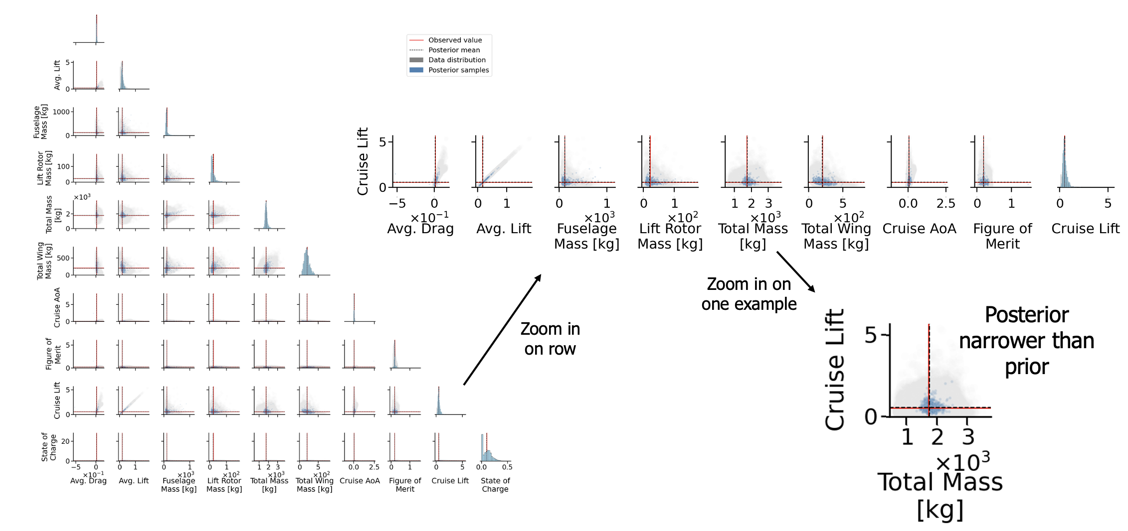
_{Posterior Predictive Check Result: The key result is that posterior samples (blue) narrow around the objective (red), illustrating that the samples generated by the MixeDiT-MaskeDiT pipeline closely match the desired objective. The gray samples represent the prior before conditioning on $\mathbf{x}$.}

---

Pictures of planes

In the paper we describe a few case studies showing how the MixeDiT-MaskeDiT design pipeline successfully captures some underlying physical laws that it has learnt from the data. Here I just include the last one that we refer to as Case Study D, where we vary the drag.

---

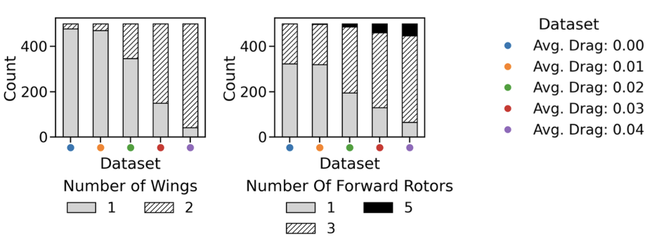
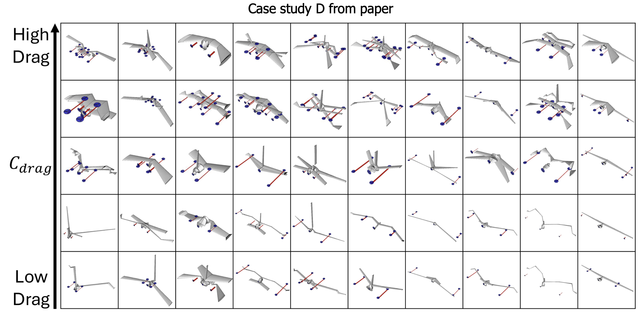
_{As we increase drag, we see an increase in the number of designs with a second wing and an increase of forward rotors. Roughly speaking, conditioning on designs with higher drag has led to designs with more components.}

---

Final comments

Overall this work introduces an SBI-inspired approach to aircraft design. The novelty comes from the hierarchical structure and the two new models of MixeDiT and MaskeDiT. More details are available in the paper as well as a link to the dataset and code.

---

Written on March 6th, 2026 by Adam Cobb